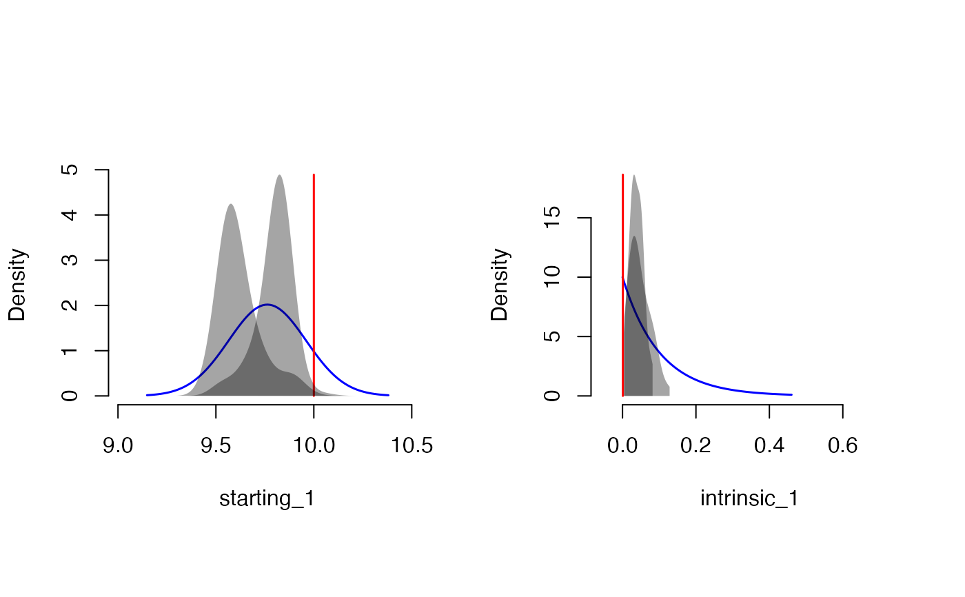
For each free parameter in the posterior, this function creates a plot of the distribution of values estimated in the last generation. This function can also be used to visually compare against true (generating) parameter values in a simulation.
plotPosteriors(
  particleDataFrame,
  priorsList,
  realParam = FALSE,
  realParamValues = NA
)
Arguments
| particleDataFrame | A |
|---|---|
| priorsList | A |
| realParam | If |
| realParamValues | Values for real parameters, include a value for each
parameter (including fixed values). Otherwise should be |
Value
Returns a plot for each free parameter.
Note
realParam and realParamValues should only be used with simulated data, where
the true values are known.
See also
plotPrior for a set of functions for visualizing and summarizing
prior and posterior distributions, including a visual comparison for single parameters.
Author
Barb Banbury and Brian O'Meara
Examples
data(simRunExample)

# make a list of particleDataFrames to plot multiple runs
resultsPDFlist <- lapply(resultsBMExample, function(x) x$particleDataFrame)

plotPosteriors(
   resultsPDFlist,
   priorsList = resultsBMExample[[1]]$priorList,
   realParam = TRUE,
   realParamValues = c(ancStateExample, genRateExample)
   )