Test If an Outlier Is Within a Highest Density Region of a Multivariate Cloud of Data Points
Source:R/testMultivarOutlierHDR.R
testMultivarOutlierHDR.RdThis function takes a matrix, consisting of multiple observations
for a set of variables, with observations assumed to be independent
and identically distributed, calculates a highest density interval
for each of those variables (using
highestDensityInterval), and then tests if some
potential 'outlier' (a particular observation for that set of
variables), is within that highest density interval.
Typically, users may want to account for possible non-independence
of the variables, which could lead to inflated false-positive rates
with this test of coverage. To account for this, this function
allows for the option of applying principal component analysis to
rotate the variables, and then calculate the highest density
intervals from the orthogonal principal component scores.
testMultivarOutlierHDR(
  dataMatrix,
  outlier,
  alpha,
  coda = FALSE,
  verboseMultimodal = FALSE,
  pca = TRUE,
  ...
)
Arguments
| dataMatrix | A matrix consisting of rows of data observations, with one or more variables as the columns, such that each multivariate observation can be reasonably assumed to represent independent, identically-distributed random variables. For example, a matrix of sampled parameter estimates from the post-burnin posterior of a Bayesian MCMC. |
|---|---|
| outlier | A vector of consisting of a single observation of one or more variables, with the same length as the number of columns in /codedataMatrix. Not necessarily a true 'outlier' per se but some data point of interest that you wish to test whether it is inside some given probability density estimated from a sample of points. |
| alpha | The threshold used for defining the highest density frequency cut-off. If the highest density interval is applied to a Bayesian MCMC posterior sample, then the interval is effectively calculated for this value as a posterior probability density. |
| coda | Default is |
| verboseMultimodal | If |
| pca | If |
| ... | Additional arguments passed to |
Value
A logical, indicating whether the given data point (outlier)
is within the multivariate data cloud at the specified threshold
probability density.
Details
Quantiles, or highest density intervals are essentially a univariate concept. They are calculated independently on each variable, as if each variable was independent. They are often used to try to piece together 'regions' of confidence or credibility in statistics. Unfortunately, this means that that if variables are correlated, the box-like region they describe in the multivariate space may not cover enough of the actual data scatter, while covering lots of empty space.
There are several solutions. There are a number of approaches for fitting ellipsoids to bivariate data. But what about multivariate datasets, such as sets of parameter estimates from the posterior of a Bayesian analysis, which may have an arbitrary number of variables (and thus dimensions)?
A different solution, applied here when pca = TRUE,
is to remove the non-independence among variables
by rotating the dataset with principal components analysis.
While this approach has its own flaws, such as assuming that the data
reflects a multivariate normal. However, this is absolutely an
improvement on not-rotating, particularly if being
done for the purpose of this functon, which is essentially to measure
coverage--to measure whether some particular set of values falls within a highest
density region (a multivariate highest density interval).
See also
This function is essentially a wrapper for applying highestDensityInterval to
multivariate data, along with princomp in package stats.
Author
David W. Bapst
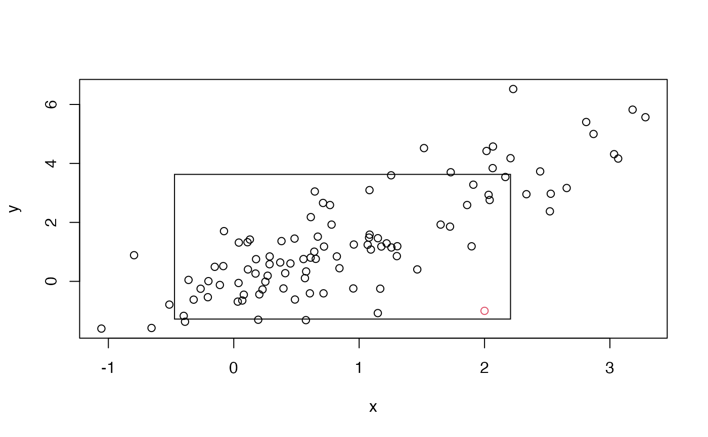
Examples
# First, you should understand the problems # with dealing with correlated variables and looking at quantiles # simulate two correlated variables set.seed(444) x <- rnorm(100, 1, 1) y <- (x*1.5)+rnorm(100) # find the highest density intervals for each variable pIntX <- highestDensityInterval(x, alpha = 0.8) pIntY <- highestDensityInterval(y, alpha = 0.8) # These define a box-like region that poorly # describes the actual distribution of # the data in multivariate space. # Let's see this ourselves... xLims <- c(min(c(x, pIntX)), max(c(x, pIntX))) yLims <- c(min(c(y, pIntY)), max(c(y, pIntY))) plot(x, y, xlim = xLims, ylim = yLims)# So, that doesn't look good. # Let's imagine we wanted to test if some outlier # was within that box: outlier <- c(2, -1) points(x = outlier[1], y = outlier[2], col = 2)# we can use testMultivarOutlierHDR with pca = FALSE # to do all of the above without visually checking testMultivarOutlierHDR(dataMatrix = cbind(x, y), outlier = outlier, alpha = 0.8, pca = FALSE)#> Warning: Less than 10 observations are given as input - estimates of the highest density region may be very imprecise#> [1] TRUE# Should that really be considered to be within # the 80% density region of this data cloud? ##### # let's try it with PCA pcaRes <- princomp(cbind(x, y)) PC <- pcaRes$scores pIntPC1 <- highestDensityInterval(PC[, 1], alpha = 0.8) pIntPC2 <- highestDensityInterval(PC[, 2], alpha = 0.8) # plot it xLims <- c(min(c(PC[, 1], pIntPC1)), max(c(PC[, 1], pIntPC1))) yLims <- c(min(c(PC[, 2], pIntPC2)), max(c(PC[, 2], pIntPC2))) plot(PC[, 1], PC[, 2], xlim = xLims, ylim = yLims)# That looks a lot better, isnt' filled with lots of # white space not supported by the observed data. # And now let's apply testMultivarOutlierHDR, with pca = TRUE testMultivarOutlierHDR(dataMatrix = cbind(x, y), outlier = outlier, alpha = 0.8, pca = TRUE)#> Warning: Less than 10 observations are given as input - estimates of the highest density region may be very imprecise#> [1] FALSE##################### # Example with four complex variables # including correlated and multimodal variables x <- rnorm(100, 1, 1) y <- (x*0.8)+rnorm(100) z <- sample(c(rnorm(50, 3, 2), rnorm(50, 30, 3))) a <- sample(c(rnorm(50, 3, 2), rnorm(50, 10, 3)))+x^2 #plot(x, y) #plot(x, z) #plot(x, a) data <- cbind(x, y, z, a) # actual outlier, but maybe not obvious if PCA isn't applied outlier <- c(2, 0.6, 10, 8) # this one should appear to be an outlier (but only if PCA is applied) testMultivarOutlierHDR(dataMatrix = data, outlier = outlier, alpha = 0.8)#> Warning: Less than 10 observations are given as input - estimates of the highest density region may be very imprecise#> [1] FALSEtestMultivarOutlierHDR(dataMatrix = data, outlier = outlier, alpha = 0.8, pca = FALSE)#> Warning: Less than 10 observations are given as input - estimates of the highest density region may be very imprecise#> [1] FALSE# this one should be within the 80% area outlier <- c(1, 0, 30, 5) testMultivarOutlierHDR(dataMatrix = data, outlier = outlier, alpha = 0.8)#> Warning: Less than 10 observations are given as input - estimates of the highest density region may be very imprecise#> [1] TRUEtestMultivarOutlierHDR(dataMatrix = data, outlier = outlier, alpha = 0.8, pca = FALSE)#> Warning: Less than 10 observations are given as input - estimates of the highest density region may be very imprecise#> [1] TRUE# this one should be an obvious outlier no matter what outlier <- c(3, -2, 20, 18) # this one should be outside the 80% area testMultivarOutlierHDR(dataMatrix = data, outlier = outlier, alpha = 0.8)#> Warning: Less than 10 observations are given as input - estimates of the highest density region may be very imprecise#> [1] FALSEtestMultivarOutlierHDR(dataMatrix = data, outlier = outlier, alpha = 0.8, pca = FALSE)#> Warning: Less than 10 observations are given as input - estimates of the highest density region may be very imprecise#> [1] FALSE